Nested watershed modeling
Model the reach, catchment, or management area you actually study — not the whole basin above it.
Four places you can cut a model
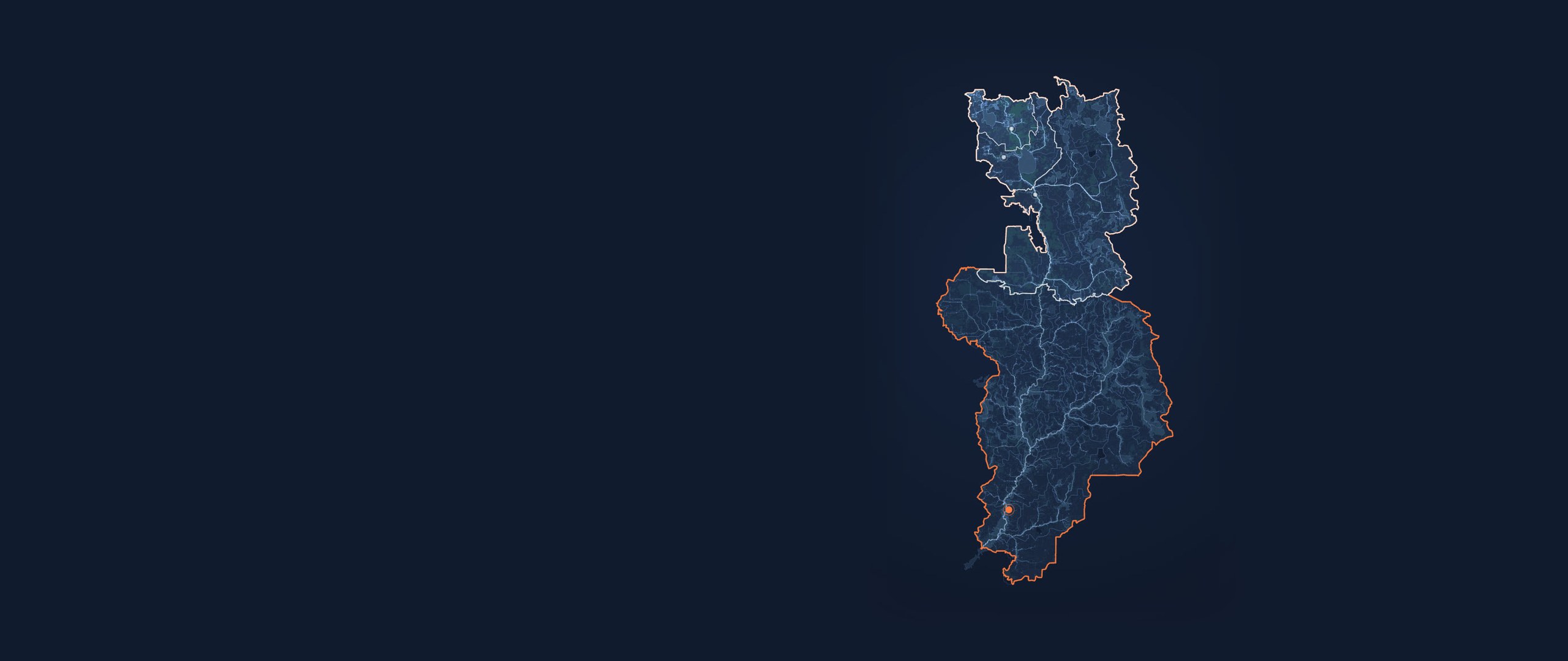
A nested study is really a choice of boundary. SWATGenX builds at all four of them.
- HUC8 subbasin
A whole 8-digit basin — the usual parent for regional water balance.
- Gauged station
The twelve-digit unit that contains a USGS stream gauge, with every unit upstream of it.
- HUC12 outlet
The watershed above any 12-digit outlet you pick in the Watershed Explorer.
- HUC14 catchment
A single catchment — site scale, where a plume, wellfield, or permit lives.
A note on gauges. Where a gauge sits on the boundary, that is the most useful cut: it comes with an observed record, so the hand-off between models is something you can check rather than something you assume.
When nesting is the wrong tool
Cutting a model is a physical claim: that nothing you care about crosses the cut in both directions. Four cases where that claim fails.
Backwater or tidal influence at the downstream boundary. A one-way boundary cannot represent water that pushes back upstream.
Upstream–downstream feedback — reservoir operation, or upstream allocation responding to downstream demand. Cutting the model hard-codes the upstream response you were trying to study.
Reactive or long-residence constituents where the reach start is arbitrary. The boundary concentration then carries the answer, and the study measures its own boundary condition.
Groundwater-dominated reaches where the aquifer crosses your cut. A surface-water boundary says nothing about where the contributing aquifer begins — this is the one most often missed.
The last one is the quiet failure. Nesting at a stream gauge cuts the stream network; it does not cut the aquifer. If lateral groundwater inflow crosses your boundary, a surface-water hand-off does not represent it, and the interior model will attribute that water to local processes. Where that matters, the boundary you need is the site-scale nested build with an explicit groundwater domain rather than a stream inlet.
Common questions
How do I model part of a large watershed without modeling the whole upstream basin?
Cut the model at a boundary you can defend, and supply what the upstream area would have contributed rather than simulating it. In practice that means one of three things: rebuild the interior as a nested model whose parent supplies its boundary conditions; hand the interior model an upstream discharge and load series at its inlet; or, where the relevant boundary is vertical rather than lateral, couple to a groundwater model. The choice is a modeling decision, not a software setting — the deciding question is whether the process you are studying crosses the boundary you want to cut.
What is nested watershed modeling?
Nested modeling runs a coarser model over a large basin and a finer model over the interior area of interest, with the coarse model supplying the fine model’s boundary conditions. It keeps resolution and data effort where the question is, instead of spending both uniformly across a basin that may be many times larger than the study area. The nesting can be horizontal (a reach or catchment inside a basin) or vertical (a three-dimensional groundwater domain inside a surface water balance).
Can I use an observed gauge record as the upstream boundary?
Yes, and it is usually the better choice when a gauge exists at your boundary. A modeled boundary carries the upstream model’s error into your interior model, and calibrating the interior then absorbs that error into local parameters — which are the parameters the study is about. An observed record removes that path entirely. This is why gauged stations are the most useful cut point: the boundary comes with its own verification data.
Does SWAT+ support inlets for upstream boundary conditions?
SWAT+ represents an inlet as a recall object. Two practical constraints apply on current releases. SWAT+ Editor 4.0.1 does not write recall files at all — the recall slot in file.cio is written as the literal token "null" — and upstream directs users who need recall to Editor 3.2.x with engine revision 61.0.2. Where recall files do exist, a yearly record is the reliable path; sub-annual records should be verified rather than assumed. The verification is simple: run with and without the boundary and difference the two runs at the channel immediately below it. If the difference is exactly zero, the boundary is not being delivered.
How many models do I need for a nested study?
Two is the common case — a parent that establishes the boundary and a child that carries the study. More than two is worth it when you want to test how sensitive your answer is to where the boundary was cut, which is done by moving the cut and rerunning rather than by argument. SWATGenX builds each model from national datasets, so adding a second or third cut point costs a build rather than a data-assembly project.