Automated U.S. watershed modeling
Role-aware PSO Calibration | SWATGenX
SWATGenX initializes scenarios, calibrates hydrology against USGS streamflow using a role-aware particle swarm optimization workflow, validates holdout periods, and summarizes uncertainty with ensemble diagnostics.
- Role-aware PSO calibration
- Mentor, mentee & independent particles
- Holdout validation
- Ensemble uncertainty diagnostics
Motivation
SWATGenX first creates a default SWAT+ (SWAT Plus) model from national hydrography, soils, land cover, terrain, and climate datasets. For Pro calibration workflows, the platform then prepares the model for hydrologic calibration by improving selected management inputs, applying crop rotation and irrigation context where national data support it, and calibrating streamflow response against USGS observations using the engine described below—not a generic parameter-tuning wrapper.
The current hosted calibration workflow is focused on hydrology and routing. It optimizes simulated streamflow against observed USGS daily discharge records. Nitrogen, phosphorus, and sediment outputs may still be produced by SWAT+, but they are not currently calibrated against observed water-quality data in this automated workflow (see What this method does not claim).
Validation is performed on a separate holdout period. Instead of reporting only one best run, SWATGenX evaluates a group of high-performing parameter sets and summarizes uncertainty using ensemble-based diagnostics.
Calibration uses USGS daily streamflow observations where overlapping records are available. Because the national climate inputs used by SWATGenX are currently built for the 2000–2024 period, calibration, warm-up, and validation windows must fall within that time range where data exist. For data provenance and flood screening, see Methodology. For workflows and Pro options, see How it works and Access levels.
Methods
Scientific basis
SWATGenX’s calibration workflow is based on a powerful swarm-based optimization. It builds on the calibration strategy developed in Rafiei et al. (2022), which introduced an improved particle swarm approach for high-dimensional, nonlinear integrated groundwater–surface water models. In SWATGenX, the same idea is adapted for scalable SWAT+ hydrologic calibration: particles search the parameter space, retain local and global memory, and are organized into behavioral roles to balance exploitation and exploration—an MMPSO-style (multi-memory particle swarm optimization) role-aware formulation suited to expensive simulation budgets.
Related publication: Rafiei, V., Mushtaq, S., Bailey, R. T., & An-Vo, D.-A. (2022). An improved calibration technique to address high dimensionality and non-linearity in integrated groundwater and surface water models. Environmental Modelling & Software, 149, 105312.
SWATGenX reports SWAT-CUP-style uncertainty diagnostics such as P-factor and R-factor, but the optimizer itself is SWATGenX’s PSO-based workflow, not SUFI-2.
Scenario initialization
Scenario initialization prepares the generated SWAT+ model before calibration. The default model is copied into an initialized working scenario, and selected agricultural management inputs are updated where the available national datasets provide enough information.
This step is designed to reduce unrealistic generic crop assumptions before calibration begins. The goal is not to change watershed geometry or the stream network, but to make land management inputs more consistent with observed agricultural patterns.
- Crop rotation context: SWATGenX uses CropScape CDL information to identify dominant agricultural rotation patterns where cropland HRUs are available. Eligible HRUs are reassigned from generic agricultural land use to rotation-specific land-use and management schedules.
- Management schedules: The initializer creates matching SWAT+ plant community and management schedule entries so that added rotations remain compatible with SWAT+ project conventions.
- Irrigation context: Where USGS HUC12 consumptive-use information indicates meaningful irrigation demand, SWATGenX can add irrigation decision logic based on plant water stress. Irrigation depth and annual application limits remain configurable.
- What remains unchanged: Scenario initialization does not alter watershed boundaries, stream topology, soils, weather inputs, or core project geometry. It mainly improves the linkage between land use, crop management, and optional irrigation.
Water use and irrigation
SWATGenX can use HUC12-scale USGS water-use information to support irrigation initialization. When the data indicate relevant agricultural water use, the platform adds irrigation operations and decision-table logic to the initialized SWAT+ scenario.
This allows irrigation to respond to modeled plant water stress rather than applying a fixed generic assumption everywhere. Users can also disable irrigation initialization when they want to compare calibrated results with and without this management adjustment.
Calibration setup & parameter bounds
The calibration workflow uses a parameter-control file that defines which SWAT+ parameters may be adjusted, the allowable range for each parameter, and how the sampled value is applied to the model input files.
Before each simulation, SWATGenX updates the selected SWAT+ input tables, sets the simulation period and warm-up years, runs the model, and compares simulated streamflow with USGS observations.
The hosted web-calibration template currently includes 41 hydrology and routing-related parameters covering basin behavior, snow processes, channels, aquifers, reservoirs, and wetlands. The table below shows the parameter bounds and update operations used by the hosted calibration workflow.
| Parameter | SWAT+ file | Min | Max | Operation | Abs. min | Abs. max |
|---|---|---|---|---|---|---|
cn_froz | parameters.bsn | 0.000862 | 0.1 | replace | — | — |
perco | hydrology.hyd | 0.3 | 3.0 | power | 0.0 | 1.0 |
epco | hydrology.hyd | 0.4 | 0.7 | replace | 0.0 | 1.0 |
esco | hydrology.hyd | 0.7 | 0.95 | replace | 0.0 | 1.0 |
cn3_swf | hydrology.hyd | 0 | 1 | replace | 0.0 | 1.0 |
frac_dc_imp | urban.urb | -90 | 5 | percentage | 0.0 | 1.0 |
frac_imp | urban.urb | -70 | 5 | percentage | 0.05 | 1.0 |
urb_cn | urban.urb | -25 | 0 | percentage | 82.0 | 98.0 |
urban_cn_a | cntable.lum | -30 | 5 | percentage | 82.0 | 98.0 |
urban_cn_b | cntable.lum | -30 | 5 | percentage | 82.0 | 98.0 |
urban_cn_c | cntable.lum | -30 | 5 | percentage | 82.0 | 98.0 |
urban_cn_d | cntable.lum | -30 | 5 | percentage | 82.0 | 98.0 |
tmp_lag | snow.sno | 0.01 | 2 | replace | — | — |
fall_tmp | snow.sno | -5 | 5 | replace | -5.0 | 5.0 |
melt_tmp | snow.sno | -5 | 5 | replace | -5.0 | 5.0 |
melt_min | snow.sno | 0 | 10 | replace | 0.0 | 10.0 |
melt_max | snow.sno | 0 | 10 | replace | 0.0 | 10.0 |
k | hyd-sed-lte.cha | 0.1 | 20 | replace | 0.0 | 500.0 |
mann | hyd-sed-lte.cha | 0.001 | 0.2 | replace | 0.0 | 0.3 |
surq_lag | parameters.bsn | 0.05 | 2.0 | replace | 0.05 | 24.0 |
gw_flo | aquifer.aqu | 0 | 1000 | multiply | 0.0 | — |
alpha_bf | aquifer.aqu | 1 | 18 | multiply | 0.0 | 1.0 |
flo_min | aquifer.aqu | 0 | 3 | multiply | 0.0 | 50.0 |
bf_max | aquifer.aqu | 0.0001 | 20 | replace | 0.1 | 2.0 |
dep_wt | aquifer.aqu | -2 | 5 | add | 0.0 | 50.0 |
dep_bot | aquifer.aqu | -5 | 15 | add | 1.0 | 50.0 |
revap_min | aquifer.aqu | 0.1 | 10 | multiply | 0.0 | 50.0 |
spec_yld | aquifer.aqu | 0.05 | 0.4 | replace | 0.0 | 0.5 |
vol_es | hydrology.res | -50 | 50 | percentage | 0.0 | — |
vol_ps | hydrology.res | -50 | 50 | percentage | 0.0 | — |
evap_co | hydrology.res | -20 | 20 | percentage | 0.0 | 1.0 |
area_ps | hydrology.res | -50 | 50 | percentage | 0.0 | — |
area_es | hydrology.res | -50 | 50 | percentage | 0.0 | — |
hru_ps | hydrology.wet | -50 | 50 | percentage | 0.0 | — |
dp_ps | hydrology.wet | -50 | 50 | percentage | 0.0 | — |
hru_es | hydrology.wet | -50 | 50 | percentage | 0.0 | — |
dp_es | hydrology.wet | -50 | 50 | percentage | 0.0 | — |
vol_area_co | hydrology.wet | -50 | 50 | percentage | 0.0 | — |
vol_dp_a | hydrology.wet | -50 | 50 | percentage | 0.0 | — |
vol_dp_b | hydrology.wet | -50 | 50 | percentage | 0.0 | — |
hru_frac | hydrology.wet | -50 | 50 | percentage | 0.0 | 1.0 |
These parameters are used to improve streamflow simulation skill. They are not intended to represent a full nutrient, sediment, or crop-yield calibration. Studies focused on water quality should apply additional manual or external calibration after downloading the model.
Objective function & performance metrics
Each candidate parameter set produces a full SWAT+ simulation. Optimization is driven by streamflow agreement against USGS daily discharge at available gaging stations: simulated channel flow is aligned in time with observed records for scoring.
The objective function emphasizes daily and monthly Nash–Sutcliffe efficiency (NSE) so that parameter sets with stronger streamflow agreement at both time scales rank higher. This is the primary basis for comparing candidates during calibration.
MAPE, PBIAS, RMSE, and KGE are computed as additional diagnostics for reporting and interpretation. They help characterize bias, relative error, and overall agreement, but they are supporting metrics alongside NSE—not the sole scientific claim of the optimizer.
Results and discussion
Role-aware particle swarm optimization
Initial candidate parameter sets are generated using Latin Hypercube Sampling across the allowed bounds. The best-performing initial candidates seed the active calibration swarm.
Each particle maintains a local best position and score, while the swarm tracks a global best. Particles are assigned one of three roles based on how their local best compares with the rest of the swarm: mentor (high-performing), mentee (lower-performing), and independent (middle-performing). Mentor, mentee, and independent particles use different velocity-update weightings: mentees are pulled more strongly toward global knowledge, while independent particles retain stronger local exploration. This role-aware structure is designed to reduce premature convergence and improve search behavior in high-dimensional, nonlinear calibration—it does not guarantee a global optimum.
The workflow is designed for computationally expensive watershed models. Simulations can be evaluated in parallel, failed runs can be retried or re-sampled when possible, and compatible previous runs canwarm-start a new calibration from checkpoints.
For a technical benchmark on single forward-model wall time on a ~94k-HRU model—and what we tried in the Fortran binary—see SWAT+ runtime benchmark on real watershed models.
Stopping rules include the maximum number of iterations, lack of improvement in the global best score, and stability of recent best-performing solutions.
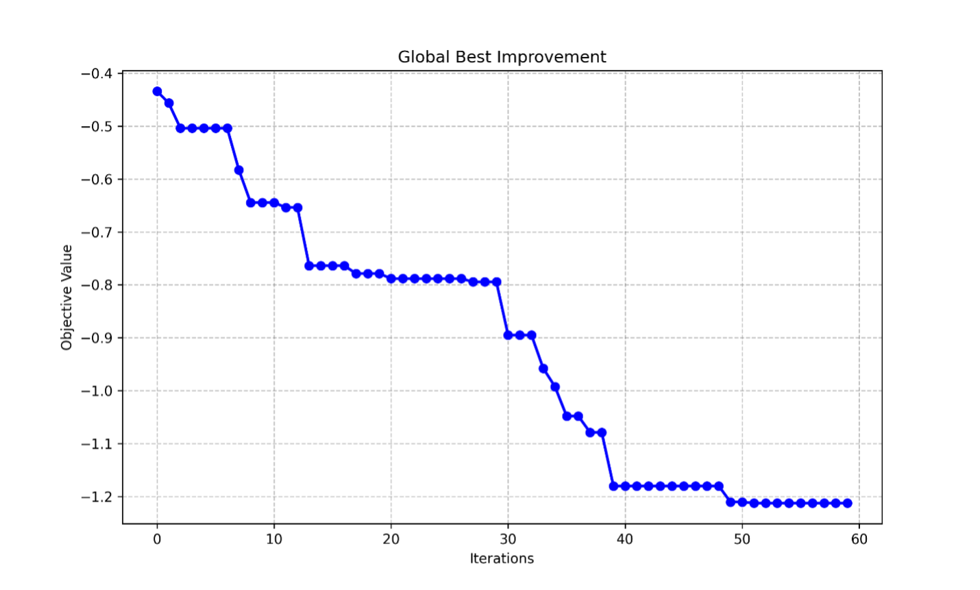
Example improvement in the global-best objective value during SWAT+ calibration. Lower objective values indicate stronger combined daily and monthly streamflow performance under the optimizer’s scoring convention.
Multi-memory PSO (MMPSO): escaping the convergence plateau
The role-aware swarm above still steers toward a single global best, so once that best lands in a local optimum the swarm converges onto it and stops improving. SWATGenX’s default optimizer is now MMPSO (multi-memory particle-swarm optimization), adapted from a published technique: it decomposes the objective by gauge and gives each particle a memory per sub-objective, so the swarm keeps exploring and breaks through that plateau. The legacy single-objective PSO remains available as a one-flag fallback. The panel below is a controlled head-to-head on the same model, seed, window, and iteration budget.
What changed and why it matters
- SWATGenX’s default auto-calibrator is now MMPSO (multi-memory particle-swarm optimization), an adaptation of a published technique that escapes the local-optimum plateau where ordinary single-objective PSO stalls.
- In a controlled head-to-head on the same model, seed, window and budget, single-objective PSO flattened by iteration 17 and self-terminated; MMPSO broke through the plateau and kept improving to iteration 50.
- MMPSO wins on every calibration metric — daily NSE, monthly NSE, water-balance (PBIAS) and KGE — with the largest gain in water balance.
- The gain comes from the algorithm, not more compute: identical particle count and iteration budget. Legacy single-objective PSO remains available as a one-flag fallback.
The method
Why single-objective PSO plateaus — and how MMPSO escapes
Ordinary PSO collapses every gauge’s daily and monthly fit into one number and steers the whole swarm toward a single best particle. Once that best lands in a local optimum the swarm converges onto it and stops improving — the flat tail you see below. MMPSO decomposes the objective and gives the swarm the structure to keep exploring.
The total objective is split into per-gauge sub-objectives, and every particle remembers its best position for each one — not a single global best. The swarm carries many partial solutions instead of collapsing to one.
Each iteration the swarm is re-split by fitness and spread into mentors (exploit), independents (the core — pulled toward a per-sub-group local best), and mentees (explore — they follow a random mentor with stochastic switches).
Mentors/mentees use random inertia and independents rank-based inertia, sustaining exploration; the early-stop that terminated single-PSO at the plateau is replaced by a no-advancement budget so the escape has room to happen.
The evidence
Convergence — single-PSO plateaus, MMPSO escapes
Controlled head-to-head on USGS 14161500 — McKenzie River, OR (4 gauges) — pool 12 · 50 iterations · seed 42 · identical for both arms; calibration 2016–2022 (2-yr warm-up), validation 2010–2015.
Global-best total NSE (daily + monthly, higher is better) per PSO iteration, from each run’s GlobalBestImprovement.csv. Both arms share the same seed, so they start identically; single-PSO flattens early and self-terminates, while MMPSO is briefly behind (more exploration) before overtaking and climbing past the plateau.
Final calibration fit (main gauge, station 2)
| Metric | Single-objective PSO | MMPSO |
|---|---|---|
| Daily NSE | 0.799 | 0.812 |
| Monthly NSE | 0.928 | 0.933 |
| PBIAS (%) | 5.260 | 1.250 |
| KGE (daily) | 0.840 | 0.851 |
| Objective (−Σ NSE, lower better) | -1.7274 | -1.7449 |
Both runs calibrated the same model over the same window; MMPSO improves every metric. The NSE deltas are modest because this basin was already well-behaved — the decisive result is the convergence behaviour above.
- This is one controlled head-to-head on a well-behaved 4-gauge basin; the magnitude of the NSE gain will vary by basin. The robust, repeatable finding is the convergence behaviour: single-objective PSO self-terminates at a plateau that MMPSO escapes.
- MMPSO is the default for new calibrations; the legacy single-objective PSO is retained and selectable for reproducibility. Both run on the same dedicated-EC2 cloud-calibration pipeline.
- MMPSO’s multi-memory is most powerful on multi-gauge basins; single-gauge models fall back to a daily/monthly split or to standard PSO behaviour, so they are never worse off.
Method after Rafiei et al., Environmental Modelling & Software 149 (2022) 105312. swatplus-rev.61.x (production) · last updated 2026-06-14.
Validation & verification (holdout ensemble)
After calibration, SWATGenX validates the model on a separate holdout period. Validation draws on high-performing parameter sets from calibration, including the global-best solution, rather than trusting a single arbitrary draw from the search history.
The ensemble view matters because hydrologic calibration is equifinal: many parameter sets can produce plausible streamflow behavior. Comparing observed streamflow with the simulated ensemble, median simulation, and best-performing member gives a more honest picture of reliability than reporting one run alone.
SWATGenX also reports SWAT-CUP-style P-factor and R-factor diagnostics for daily and monthly streamflow. These summarize how well the simulation ensemble brackets observed flows and how wide the uncertainty band is. The reporting style parallels SWAT-CUP uncertainty summaries; the underlying optimizer remains SWATGenX’s role-aware PSO workflow, not SUFI-2.
Limitations and scope
What this method does not claim
Today’s hosted workflow is hydrology and streamflow calibration. It does not automatically calibrate nutrients, sediment, PFAS, or crop yield. Water-quality or land-output calibration should be treated as a separate downstream workflow after download, with study-specific data and review.