Worked examples · real basins
Calibration Examples: Controlled Basins to Regional Fleets
How SWATGenX calibration performs on real gaged watersheds — two compact controlled basins with honest split-sample metrics (one strong, one deliberately weak), and living regional cascade examples from the west-central Florida fleet, where a pooled prior lifts a 58-gauge roster in a single uncalibrated run.
- 2 controlled basins · split-sample
- 4-basin regional campaign (west-central FL)
- Zero-shot prior: median mNSE 0.05 → 0.50
- Weak results published, not hidden
Scope and intent
These are calibration examples. The two controlled basins show how a generated SWAT+ project moves through initialization, calibration, verification, and sensitivity analysis on compact single-gauge watersheds; the regional cascade tier below shows the same platform operating at fleet scale — 57k–77k-HRU basins with rosters of dozens of gauges. None of it is intended to claim national predictive skill.
Each controlled-basin example below includes (1) a compact model identity record, (2) interactive figures sourced from the same exported artifacts used in the publication, and (3) a Morris-ranked parameter subset and split-sample metrics table for quick comparison.
Parameter bounds and transformation rules come from the SWATGenX calibration template documented on /calibration-methods. For each basin below, the calibration run uses a Morris-trimmed subset of those candidate parameters.
The two basins deliberately bracket the range. Florida is a clean rainfall–runoff watershed where the generated model, calibrated against a single daily-plus-monthly NSE objective, reaches strong split-sample skill (daily NSE 0.84 in calibration, 0.73 in independent verification). Illinois is the harder case — snowmelt- and baseflow-driven, where the same single-objective workflow is markedly weaker (daily NSE 0.37 and 0.22) and snow and groundwater parameters dominate the sensitivity ranking. We show both unedited, because an honest example set has to include where an automated calibration does and does not do well.
Methods
For each basin the model identity record and simulation/optimizer configuration document how the example was built; the calibration uses a Morris-trimmed subset of the candidate parameter template.
Controlled-basin results
Per basin: the Morris sensitivity ranking, the calibration and verification split-sample metrics, and the interactive figure switcher (calibration, verification, and sensitivity outputs).
Florida controlled basin (USGS 02297600)
Calibration station: 02297600 (gage channel 2).
Use the figure controls to compare calibration and verification performance at the same station and to see the Morris screening outcome that selected the calibration subset.
Interactive figures: switch between calibration, verification, and sensitivity outputs. Hydrograph plots include the run-stage metrics on the figure (as in the publication artifacts).
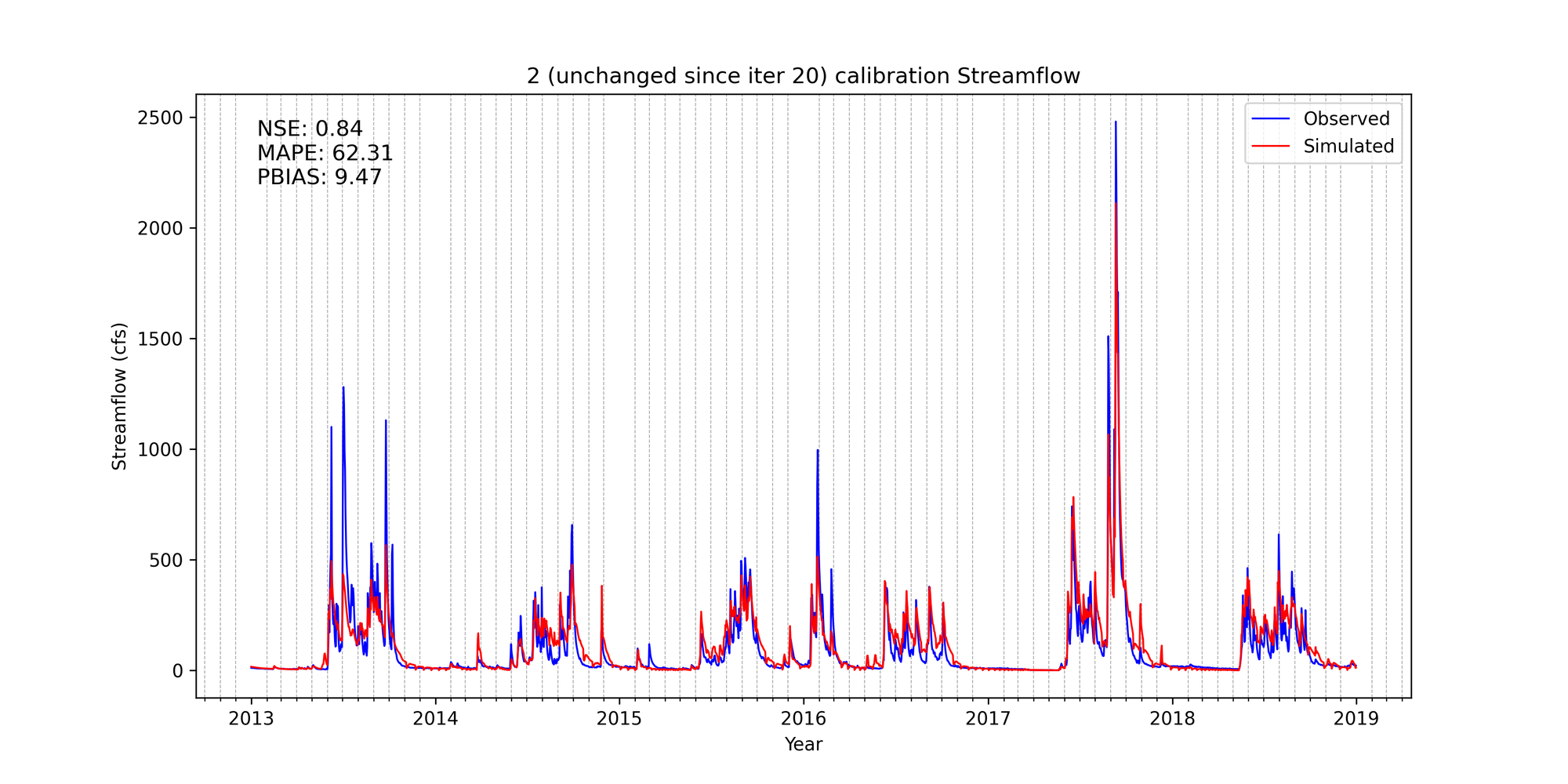
Calibration global best (daily)
- Calibration: compares the pre-optimization initialization pool and the calibrated global best for the scored calibration window.
- Verification: shows the independent holdout window results (no overlap with the scored calibration period).
- Sensitivity: Morris tornado plot used to rank candidate parameters and pick the trimmed calibration subset.
| Field | Value |
|---|---|
| Calibration station | USGS streamgage 02297600 (NHDPlus HR region 0310) |
| Scored calibration window | 2013-01-01 to 2018-12-31 |
| Independent verification window | 2019-01-01 to 2024-12-31 |
| Simulation & optimizer | Simulated 2010–2018 with a 3-year warm-up; particle-swarm optimization with 36 particles over 70 iterations, 6 run concurrently. |
Sensitivity analysis (Morris)
Morris screening runs a fixed evaluation budget and reports μ* (magnitude of the elementary effect) and σ (interaction / nonlinearity signal). The table below lists the top drivers by μ*.
| Rank | Parameter | μ* (mean effect) | σ (interaction) |
|---|---|---|---|
| 1 | surq_lag | 0.6435 | 0.4685 |
| 2 | perco | 0.288 | 0.4113 |
| 3 | cn3_swf | 0.1413 | 0.1699 |
| 4 | alpha_bf | 0.0921 | 0.0987 |
| 5 | dep_wt | 0.0882 | 0.1565 |
| 6 | spec_yld | 0.0545 | 0.0945 |
| 7 | flo_min | 0.0519 | 0.0774 |
| 8 | dp_es | 0.05 | 0.0282 |
Sensitive parameters (top 8 by μ*): surq_lag, perco, cn3_swf, alpha_bf, dep_wt, spec_yld, flo_min, dp_es.
Parameters selected for calibration in this example: 8 (the Morris-trimmed subset above). The complete candidate parameter template and bounds are documented on /calibration-methods.
Calibration and verification results
Metrics are reported for daily and monthly time steps (NSE, KGE, and PBIAS). Values below are pulled from the exported run summary tables used in the publication workflow evaluation.
| Stage | Period | Daily NSE | Monthly NSE | Daily KGE | Monthly KGE | PBIAS (%) |
|---|---|---|---|---|---|---|
| Initialization pool best | 2013–2018 | 0.795 | 0.843 | 0.68 | 0.713 | 28.127 |
| Calibration global best | 2013–2018 | 0.837 | 0.897 | 0.816 | 0.886 | 9.791 |
| Verification global best | 2019–2024 | 0.729 | 0.798 | 0.747 | 0.817 | 7.48 |
Illinois controlled basin (USGS 05536265)
Calibration station: 05536265 (gage channel 25).
Use the figure controls to compare calibration and verification performance at the same station and to see the Morris screening outcome that selected the calibration subset.
Interactive figures: switch between calibration, verification, and sensitivity outputs. Hydrograph plots include the run-stage metrics on the figure (as in the publication artifacts).
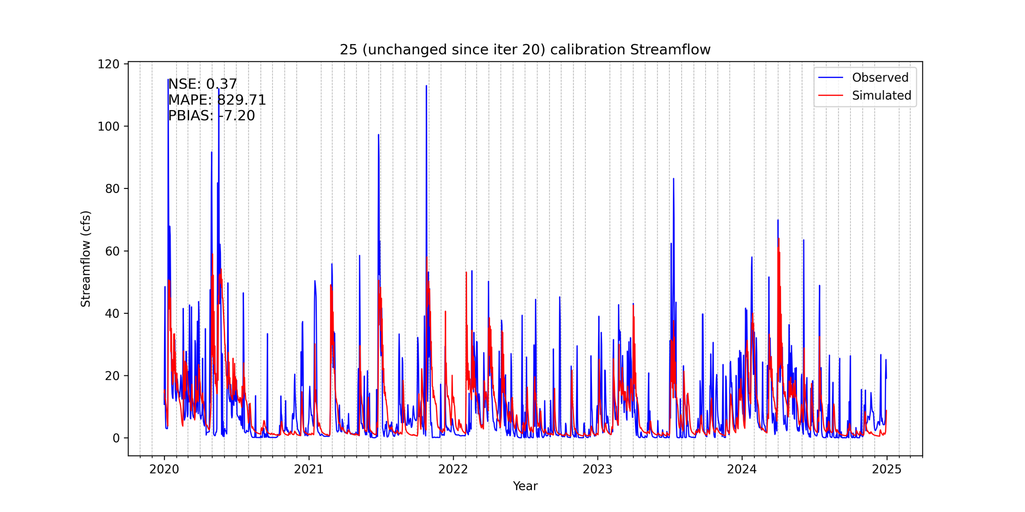
Calibration global best (daily)
- Calibration: compares the pre-optimization initialization pool and the calibrated global best for the scored calibration window.
- Verification: shows the independent holdout window results (no overlap with the scored calibration period).
- Sensitivity: Morris tornado plot used to rank candidate parameters and pick the trimmed calibration subset.
| Field | Value |
|---|---|
| Calibration station | USGS streamgage 05536265 (NHDPlus HR region 0712) |
| Scored calibration window | 2020-01-01 to 2024-12-31 |
| Independent verification window | 2012-01-01 to 2015-12-31 |
| Simulation & optimizer | Simulated 2018–2024 with a 2-year warm-up; particle-swarm optimization with 48 particles over 50 iterations, 6 run concurrently. |
Sensitivity analysis (Morris)
Morris screening runs a fixed evaluation budget and reports μ* (magnitude of the elementary effect) and σ (interaction / nonlinearity signal). The table below lists the top drivers by μ*.
| Rank | Parameter | μ* (mean effect) | σ (interaction) |
|---|---|---|---|
| 1 | melt_min | 3.82 | 9.8425 |
| 2 | k | 3.6832 | 3.7334 |
| 3 | cn3_swf | 3.3198 | 2.0242 |
| 4 | perco | 3.1507 | 4.9258 |
| 5 | melt_max | 2.9509 | 9.8071 |
| 6 | urban_cn_c | 2.8681 | 2.9149 |
| 7 | mann | 1.782 | 1.3773 |
| 8 | surq_lag | 1.7715 | 2.685 |
Sensitive parameters (top 8 by μ*): melt_min, k, cn3_swf, perco, melt_max, urban_cn_c, mann, surq_lag.
Parameters selected for calibration in this example: 8 (the Morris-trimmed subset above). The complete candidate parameter template and bounds are documented on /calibration-methods.
Calibration and verification results
Metrics are reported for daily and monthly time steps (NSE, KGE, and PBIAS). Values below are pulled from the exported run summary tables used in the publication workflow evaluation.
| Stage | Period | Daily NSE | Monthly NSE | Daily KGE | Monthly KGE | PBIAS (%) |
|---|---|---|---|---|---|---|
| Initialization pool best | 2020–2024 | 0.202 | 0.405 | 0.605 | 0.61 | 2.856 |
| Calibration global best | 2020–2024 | 0.371 | 0.6 | 0.548 | 0.792 | -7.201 |
| Verification global best | 2012–2015 | 0.223 | 0.416 | 0.442 | 0.659 | -21.581 |
Regional cascade examples (west-central Florida)
The controlled basins above are single-gauge problems. The west-central Florida fleet — Tampa Bay, Peace, Hillsborough, and Myakka, four platform-generated coupled SWAT+/MODFLOW 6 basin models — is where the calibration methodology scales up: 29k–77k-HRU models, rosters of dozens of USGS gauges, regionalized parameters, and the information-cascade workflow (pooled priors → zero-shot seeding → bounded terminal MMPSO) documented on /calibration-methods. These are living examples: the campaign is running now, and this section is updated as stages complete. The fleet’s home is the Florida nonpoint-source living page, with interactive 3D viewers for each basin (Tampa Bay, Peace, Hillsborough, Myakka).
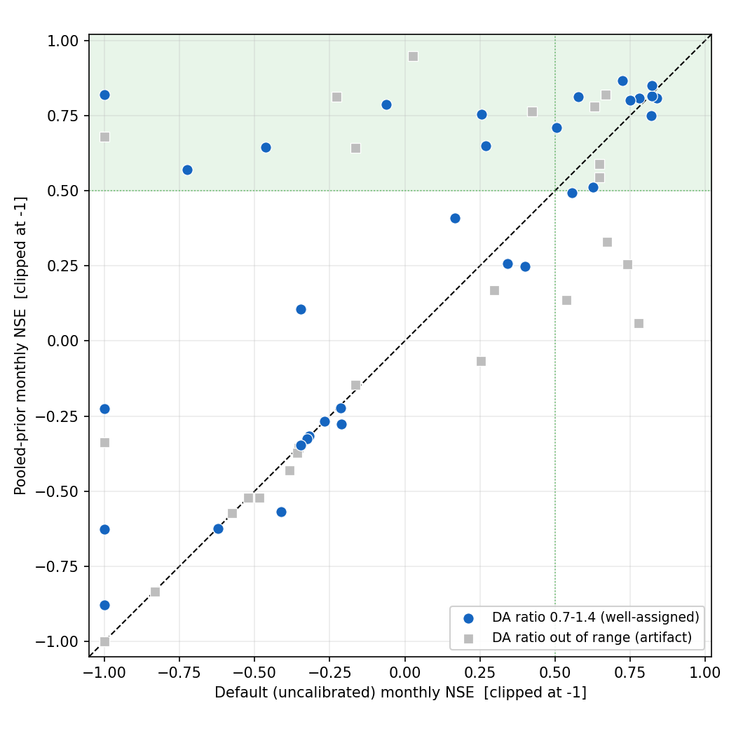
Tampa Bay: what a pooled regional prior does zero-shot
A parameter distribution pooled from previously calibrated Peace-area models was applied to the 77.6k-HRU Tampa Bay catalog model — a different basin, a different estuary — in one simulation, with no optimizer and no tuning. The scatter compares each gauge’s monthly NSE under the default (uncalibrated) parameters against the pooled prior, over the 2016–2024 scored window.
Default (uncalibrated) vs pooled-prior monthly NSE per gauge, clipped at −1 for display. Blue points are well-assigned gauges (drainage-area ratio 0.7–1.4); grey squares are assignment artifacts excluded from the honest subset. Shaded band = Moriasi Satisfactory and better. Source artifact: tampa_catalog_pooled_vs_default.png/.csv in the calibration-campaign research log.
| Gauge set | Satisfactory+ | Good+ | Very good | Median monthly NSE |
|---|---|---|---|---|
| All 58 evaluated gauges | 19 → 25 | 9 → 17 | 4 → 11 | −0.11 → +0.26 |
| Correctly-assigned subset (n=32, DA ratio 0.7–1.4) | 11 → 16 | 7 → 12 | 4 → 8 | 0.05 → 0.50 |
All values are default (uncalibrated) → pooled prior, from one 10-year simulation scored with the same evaluation pipeline as the baseline (2016–2024 window, monthly Moriasi ratings). The honest trade-off: a few small urban canals that the default happened to fit went down under the regional prior — it trades a handful of idiosyncratic gauges for large basin-wide gains. The terminal calibration stage that follows the Peace playbook has since completed on this model — its per-gauge results are below.
Peace River: the first production regionalized MMPSO calibration
Complete
The Peace River model is the fleet’s calibration flagship and the demonstration target of the information-cascade methodology (manuscript in preparation). Terminal calibration stage COMPLETE — regional MMPSO, converged at iteration 8. The terminal step — a regionalized MMPSO over only the sensitive parameters, seeded from the pooled prior — closes the cascade: prior (a pooled distribution that transfers zero-shot) → diagnosis (which parameters to move, and a calibratability screen) → a short, seeded, regional terminal search that satisfices the fixed criteria on the reaches that carry the basin.
| Field | Value |
|---|---|
| Target model | 57,998-HRU Peace River basin model (HUC8 03100101, NHDPlus HR region 0310) |
| Gauge roster | 38 evaluated → 11 structural exclusions (drainage-area mismatch, lake-outlet orphaning, regulated canals); the terminal objective couples the retained gauges as per-gauge sub-objectives — 21 returned computable NSE over the scored window |
| Regionalization | cn3_swf, perco, esco, epco expanded over 9 tributary regions — 73 optimizer dimensions (insensitive + basin-uniform parameters stay global) |
| Optimizer | MMPSO with per-gauge sub-objectives (by-gauge grouping); pooled-prior vector injected as a protected initial particle |
| Objective hardening | Per-gauge NSE floor at −1 inside the optimizer sum (reported metrics unclipped) — pathological reaches are protected in-objective and reported honestly, not hand-excluded |
| Convergence | Global best reached at iteration 8 and held byte-identical through iteration 23 (spot instance reclaimed) — 15 iterations of zero improvement; ~100 model evaluations at 12 particles |
The search converged fast: the global-best objective (−19.25 in penalized units) was reached at iteration 8 and held unchanged for the remaining 15 iterations until the AWS spot instance was reclaimed — convergence, not a truncated run. A good pooled prior plus a fixed search space places the satisficing target within ~8 iterations, at roughly 100 model evaluations against the several hundred a from-scratch campaign would spend.
Per-gauge skill (2016–2022 calibration window (daily and monthly Moriasi NSE))
| Gauge | Daily NSE | Monthly NSE | Group |
|---|---|---|---|
| 427 | 0.79 | 0.88 | Mainstem / Charlie core |
| 422 | 0.78 | 0.86 | Mainstem / Charlie core |
| 439 | 0.78 | 0.87 | Mainstem / Charlie core |
| 332 | 0.77 | 0.92 | Mainstem / Charlie core |
| 399 | 0.77 | 0.86 | Mainstem / Charlie core |
| 2718 | 0.68 | 0.77 | Mainstem / Charlie core |
| 269 | 0.64 | 0.91 | Mainstem / Charlie core |
| 451 | 0.63 | 0.76 | Mainstem / Charlie core |
| 220 | 0.39 | 0.80 | Interior tributary |
| 650 | 0.24 | 0.47 | Interior tributary |
| 968 | 0.19 | 0.12 | Lower-basin (floor-protected) |
| 603 | 0.12 | −0.27 | Lower-basin, regulated (floor-protected) |
| 933 | −0.27 | −0.49 | Tidal reach (floor-protected) |
| 947 | −2.36 | 0.53 | Tidal — daily degenerate, monthly recovers (floor-protected) |
The mainstem and Charlie Creek core — the reaches that integrate the basin’s water balance — is Good to Very Good (monthly NSE 0.86–0.92, daily 0.63–0.79). Four lower-basin and tidal gauges remain weak: the per-gauge floor is why they neither dominated the search nor were quietly dropped. Their failures are hydrologic-signal and regulation artifacts of the coastal setting (e.g. gauge 947, whose daily NSE is degenerate under tidal aliasing yet whose monthly NSE recovers to 0.53), not parametric deficits the free set could repair. They are reported at face value rather than excluded post hoc to inflate a count.
Regionalization is visible in the solution: percolation (perco) ranges from 1.98 in Horse Creek to 2.83 in Shell Creek across tributary groups (Prairie 2.79, Charlie 2.70, Peace mainstem 2.52, other 2.63) — spatially-varying calibrated parameters a single global scalar could not produce, reconciling the opposite per-tributary biases.
Per-gauge NSE above are from the best-so-far synchronized forward-run snapshot (the readable, directly-interpretable units); the assembled global-best solution is marginally better but stored in penalized units. Why the objective is floored: an earlier attempt collapsed because one pathological near-zero-flow gauge dominated a naive summed-NSE objective — the honest finding that produced the per-gauge floor and the roster discipline documented on /calibration-methods. Cost context: this class of run — a full regional calibration of a 57k-HRU model — has a measured compute cost of about $14 on AWS (see the AWS calibration page).
Cross-basin replication: the same cascade on Tampa Bay and Myakka
The cascade is designed to be basin-agnostic, so the demonstration should not rest on one basin. We ran the identical workflow — pooled prior → optimizer-free diagnosis → a short, seeded, regional terminal MMPSO — to completion on two more fleet models. Both converged from the same pooled-prior seed, giving a three-basin demonstration rather than a single case.
Tampa Bay (77.6k HRUs): terminal calibration
Complete
The zero-shot pooled prior above lifted the 58-gauge roster in one simulation; the terminal step then refines it. Terminal calibration stage COMPLETE — regional MMPSO, converged at iteration 6. This is the cross-basin case: the pooled prior carried no Tampa Bay information, yet a six-iteration regional search on a 77.6k-HRU model recovers Satisfactory-to-Very-Good skill on the reaches that carry the basin.
| Field | Value |
|---|---|
| Target model | 77,636-HRU Tampa Bay integrated model (70 HUC12s, HUC12-outlet 031002060700, region 0310) — a separate drainage feeding a nitrogen-limited estuary |
| Gauge roster | 32 gauges retained after coverage + drainage-area vetting; 27 returned computable NSE over the scored window |
| Regionalization | runoff-controlling parameters (cn3_swf, perco, esco, epco) distributed by tributary sub-watershed; snow / storage / channel / baseflow stay global |
| Optimizer | MMPSO with per-gauge NSE sub-objectives (floor −1); pooled-prior vector (built entirely from the Peace-area pool, no Tampa Bay information) injected as a protected initial particle |
| Convergence | Global best (−15.48 in penalized units) reached at iteration 6 and held byte-identical through the final synchronized iteration — a converged plateau, not a truncated run |
Per-gauge skill (2016–2022 calibration window (daily and monthly Moriasi NSE))
| Gauge | Daily NSE | Monthly NSE | Group |
|---|---|---|---|
| 817 | 0.70 | 0.85 | Well-gauged core |
| 1106 | 0.61 | 0.74 | Well-gauged core |
| 837 | 0.60 | 0.68 | Well-gauged core |
| 1671 | 0.55 | 0.62 | Well-gauged core |
| 1979 | 0.54 | 0.85 | Well-gauged core |
| 2184 | 0.53 | 0.66 | Well-gauged core |
| 844 | 0.52 | 0.64 | Well-gauged core |
| 1868 | 0.42 | 0.82 | Interior (strong monthly) |
| 1013 | 0.42 | 0.80 | Interior (strong monthly) |
| 1495 | 0.35 | 0.82 | Interior (strong monthly) |
| 1265 | −0.19 | −0.78 | Small urban canal (floor-protected) |
| 1689 | −0.28 | −0.71 | Small urban canal (floor-protected) |
| 1267 | −0.29 | −0.42 | Small urban canal (floor-protected) |
The well-gauged core is Satisfactory-to-Very-Good on the reaches that carry the basin (core daily NSE 0.52–0.70, monthly 0.62–0.85, with several interior gauges reaching monthly NSE 0.80–0.85). A cluster of seven small urban canals stays weak — their monthly PBIAS pins at roughly −100% (near-zero measured baseflow the coarse 500 m routing cannot reproduce) — and the per-gauge floor is why they neither dominated the search nor were quietly dropped. The same cascade, the same honesty rail: seeded from the pooled prior, converged in six iterations on a 77.6k-HRU model, weak tail reported at face value.
Myakka River (29k HRUs): terminal calibration
Complete
Terminal calibration stage COMPLETE — regional MMPSO, converged at iteration 5. Myakka ran against the coverage-vetted 11-gauge roster — the corrected roster after a −99 sentinel value was found and scrubbed, the same roster-discipline point documented on /calibration-methods.
| Field | Value |
|---|---|
| Target model | 29,071-HRU Myakka River model (HUC8 03100102, region 0310) — a flat wet-prairie / flatwoods basin draining to phosphorus-driven Charlotte Harbor |
| Gauge roster | 11-gauge coverage-vetted roster — the corrected roster after a −99 sentinel value was discovered and scrubbed; 10 returned computable NSE |
| Regionalization | runoff-controlling parameters distributed by tributary sub-watershed, insensitive + basin-uniform parameters global (same dispatch as Peace / Tampa Bay) |
| Optimizer | MMPSO with per-gauge NSE sub-objectives (floor −1); pooled-prior vector injected as a protected initial particle |
| Convergence | Global best (−7.03 in penalized units) reached at iteration 5 and held byte-identical through the final synchronized iteration |
Per-gauge skill (2016–2022 calibration window (daily and monthly Moriasi NSE))
| Gauge | Daily NSE | Monthly NSE | Group |
|---|---|---|---|
| 3592 | 0.40 | 0.56 | Mainstem core |
| 148 | 0.33 | 0.64 | Mainstem core |
| 191 | 0.31 | 0.65 | Mainstem core |
| 297 | 0.21 | 0.64 | Interior tributary |
| 676 | 0.25 | 0.51 | Interior tributary |
| 490 | 0.25 | 0.42 | Interior tributary |
| 220 | 0.23 | 0.31 | Interior tributary |
| 506 | 0.18 | 0.46 | Interior tributary |
| 950 | 0.17 | 0.21 | Flatwoods / low-yield |
| 433 | 0.09 | 0.19 | Flatwoods / low-yield |
Myakka is the flattest, most diffuse basin in the fleet, and its daily skill is inherently lower — but the whole coverage-vetted roster stays positive at both time scales. The core mainstem/wet-prairie gauges reach monthly NSE 0.56–0.65 (gauges 3592, 148, 191, 297), with daily NSE a modest 0.17–0.40 reflecting the flatwoods hydrology. No pathological floored tail: a fully-positive but honestly modest result from the same pooled-prior seed and the same short terminal search.
Across three basins — Peace (57,998 HRUs), Tampa Bay (77,636), and Myakka (29,071) — the same three-step cascade converged from the same pooled-prior seed in five to eight iterations, each time recovering defensible skill on the core gauges while retaining any weak reaches honestly under the per-gauge floor. That the workflow holds across a phosphorus-driven mining basin, a nitrogen-limited estuary drainage, and a flat wet-prairie river is the point: the method is basin-agnostic, now with three basins of evidence.
Notes
Notes
- Controlled-basin calibration objective: minimize the negative sum of daily NSE and monthly NSE at the gaged channel. Fleet-scale runs extend the same objective across the whole gauge roster with a per-gauge NSE floor (see calibration methods).
- Verification uses an independent window with no overlap with the scored calibration period (split-sample).
- The regional cascade tier reports platform-generated models finished by expert workflow steps; every number on this page cites its exported artifact, and in-progress stages are labeled as such.
- If you order a calibration run on your own model, the UI will show runtime/cost estimates before execution.